Every tyre is a radio station: listening to TPMS with an RTL-SDR

In the last blog, we went through what is inside a TPMS sensor and dug through its FCC filings to learn what it does and how it sends its data to the car’s control unit. We have also seen that the packets are not encrypted, and that the raw packets are broadcast on the 433.92 MHz frequency. This is the detail we will focus on for the rest of the series. We will use a cheap radio receiver to collect this data and do all sorts of interesting stuff with it.

What is an RTL-SDR?

An RTL-SDR started its life as a cheap USB TV tuner. These dongles were made to watch digital TV (DVB-T) on a laptop, and most of them use a Realtek chip called the RTL2832U. Back in 2012, a Linux kernel developer, Antti Palosaari, found that this chip can hand over the raw radio samples to the computer, not just the decoded TV picture. Soon after, the Osmocom community wrote open source drivers and tools for it, and a TV tuner turned into a software defined radio (SDR).

So what is software defined about it? In a normal radio, the hardware decides what you can listen to. An FM radio can only play FM. In an SDR, the hardware just tunes to a frequency and captures the raw signal, and the software on your computer does the rest. The same dongle can listen to FM radio, aircraft, weather satellites, or the tyres of a passing car. All you need to change is the software.

This opened up the radio world to amateurs. Before this, a receiver that could do all of this cost a lot of money. Now, anyone with a laptop and a dongle that costs a few thousand rupees can explore the radio waves around them.

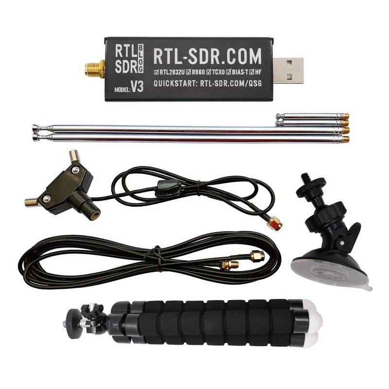The RTL-SDR Blog V3 kit, the one I use. Image: RTL-SDR Blog.

There are many RTL-SDR dongles out there. The one I have is the RTL-SDR Blog V3, which comes as a kit with a dipole antenna. In India, you can buy it from one of the resellers listed on the RTL-SDR Blog store.

How it started

I had the RTL-SDR lying around, and I was only using it for things like capturing SSTV images from the ISS and watching ADS-B messages from flights. These were simple experiments, already well documented, and lots of people have done great stuff with them. Then, I came across a paper that showed how tyre sensors can reveal a lot about your daily activity. It was an interesting read, and it caught my attention. So I read several more papers around these sensors. I was so fascinated by them that I wanted to try it out and listen to these sensors myself.

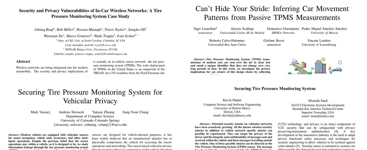Some of the papers I read on TPMS security and privacy.

Here are the papers, if you want to read them yourself:

• Security and Privacy Vulnerabilities of In-Car Wireless Networks: A Tire Pressure Monitoring System Case Study (Rouf et al., USENIX Security 2010)
• Can’t Hide Your Stride: Inferring Car Movement Patterns from Passive TPMS Measurements (Lizarribar et al., IEEE WONS 2026)
• Securing Tire Pressure Monitoring System for Vehicular Privacy (Vaszary et al., University of Colorado Colorado Springs)

rtl_433: the Shazam for radio signals

Through the papers, I came across an open source tool, rtl_433, and I was curious to try it out. All I needed was the RTL-SDR and the antenna that came with it. Since the kit comes with a telescopic dipole antenna, it can be adjusted for the 433 MHz frequency. You can use an online dipole calculator to find the length to set the antenna to. For 433.92 MHz, each side of the dipole comes to about 16.5 cm. The RTL-SDR Blog also has a guide on using the dipole kit.

The first thing I tried was to sit by the roadside. We need tyres transmitting data, and lots of them, so a busy road is the best place to be. I connected the RTL-SDR with the antenna to my laptop and started rtl_433 like this:

$ rtl_433 -f 433.92M -M level

The -f 433.92M tells it which frequency to listen on, and -M level adds the signal strength of each packet to the output. Once I started the tool and waited for a few cars to pass by, I started seeing data popping up on the screen.

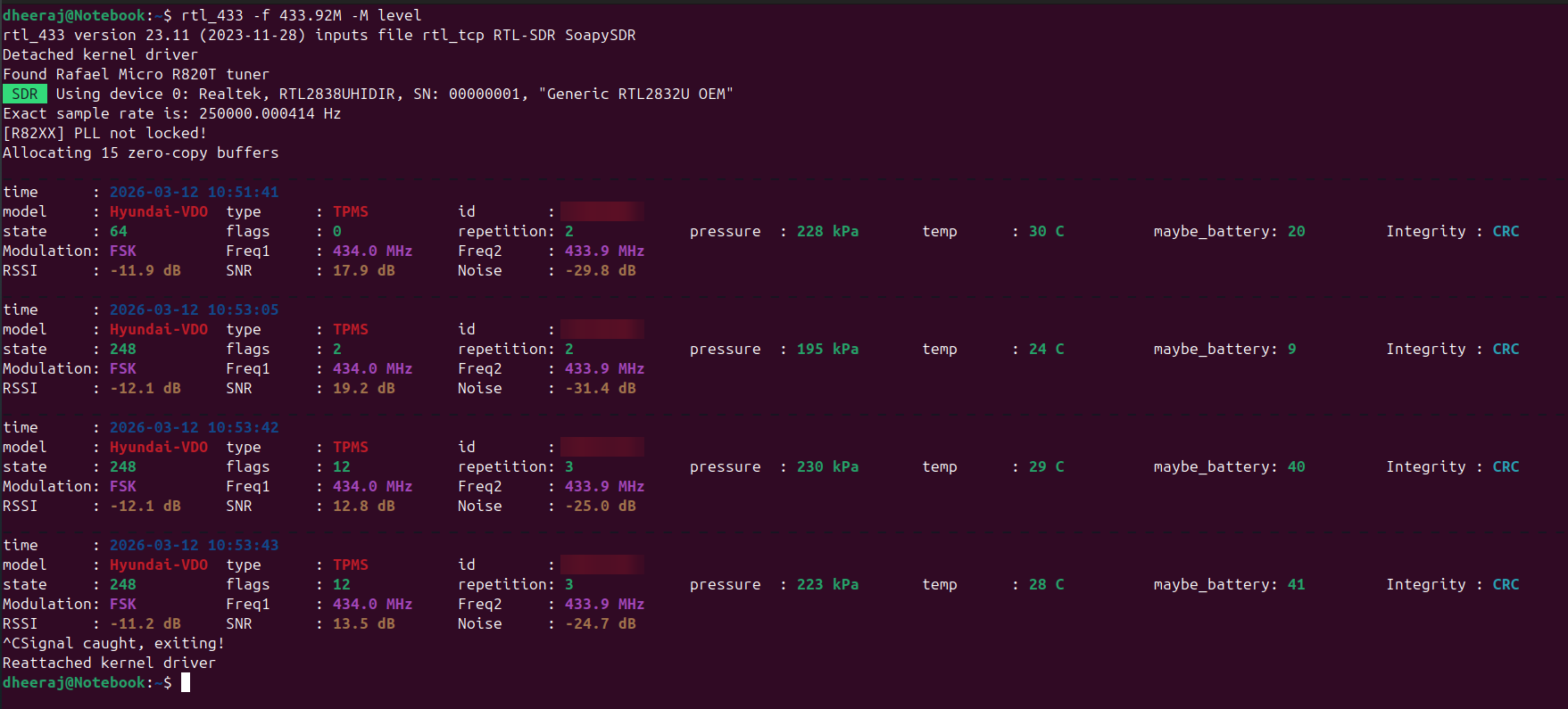My first capture by the roadside: four tyre packets from passing cars, with pressure and temperature. Sensor IDs blurred.

This was fascinating. I could see the tyre pressures and temperatures of passing cars, live, in front of me. I sat there for a while and came back home wondering how all of this works. Over the next few weeks, I took my laptop and the RTL-SDR with me whenever I went on a drive.

The passenger seat lab

I started out by keeping the laptop and the RTL-SDR setup on the passenger seat next to me and running the tool. You can see how I stuck the antenna to the window for better reception. I got all kinds of weird looks because of this while driving around the city. Initially, I was just watching the packets print on the screen as I drove. This gave me an idea of what kind of packets we can receive on a drive.

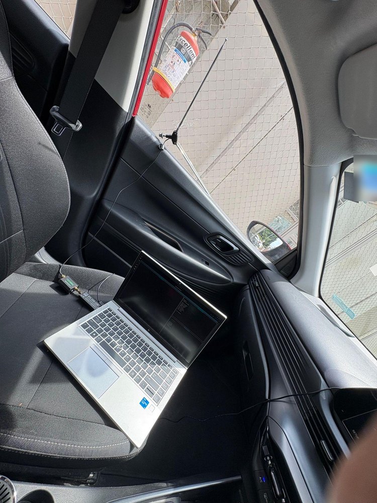The passenger seat lab: a laptop, the RTL-SDR and the antenna on the window.

I then started saving the packets to a file. rtl_433 has an option to write the packets to a JSON file, one packet per line:

$ rtl_433 -f 433.92M -M level -F json:tpms_packets.json -F kv

The -F json:tpms_packets.json writes every packet to the file, and -F kv keeps printing them on the screen as before. Each line in the file looks something like this:

{"time" : "2026-03-12 10:51:41", "model" : "Hyundai-VDO", "type" : "TPMS", "id" : "xxxxxxxx", "pressure_kPa" : 228.000, "temperature_C" : 30.000, ...}

This was helpful, as I could drive around peacefully without looking at the laptop every now and then. At the end of the day, I could go home and go through the packets.

v1.1: Collecting more data

As you might have noticed in the photo, there is another device attached to the RTL-SDR. I read online that an amplifier can increase the range and help collect more packets. So I ordered the Nooelec LaNA WB, a low noise amplifier (LNA), and immediately started seeing a huge increase in the number of packets collected.

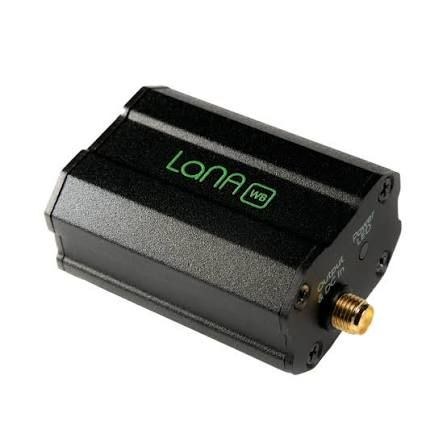The Nooelec LaNA WB amplifier. Image: Nooelec.

What did we catch?

I kept collecting data daily, on my way to work and back. After a month or so, I started thinking about doing some data analysis on it. I have now been collecting data for almost the whole year, and I’m still at it. We will see all kinds of interesting stuff and data analysis on it in a later post. For now, here is a quick look at what we caught.

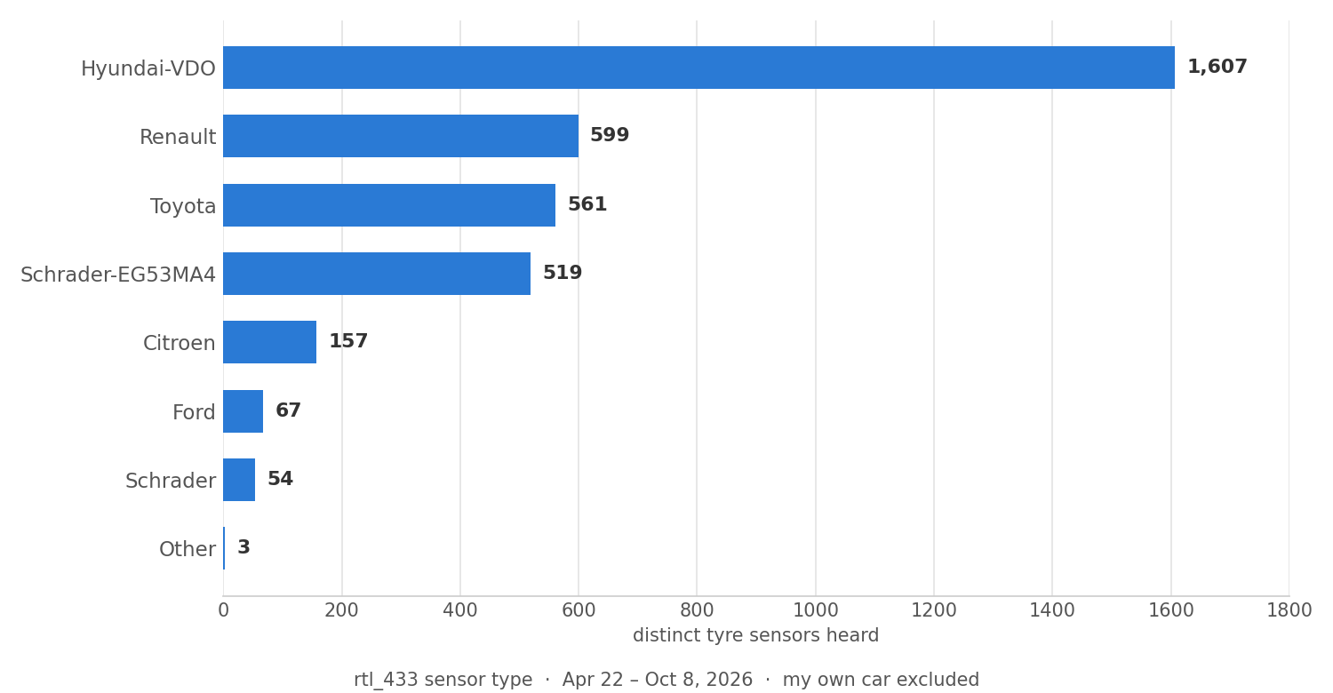Tyre sensors I heard on my drives, by the sensor type rtl_433 decoded.

As you can see in the chart, we got some useful stats. Hyundai-VDO sensors are by far the most common, followed by Renault, Toyota and Schrader. Keep in mind that these are the names of the rtl_433 decoders, which are named after the sensor or the car brand they were first found in, so they don’t map exactly to car brands. And each car has four tyres, so the number of cars is roughly a quarter of these numbers.

You can also see some other signals on the 433 MHz band. Tyres are not the only things talking on it. rtl_433 also picked up keyless entry and gate remotes, smoke detectors, burglar alarm door sensors and even household energy monitors.

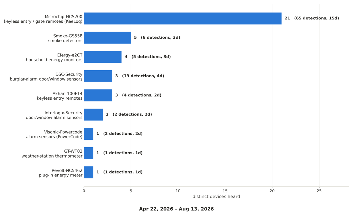Other devices rtl_433 picked up on 433 MHz between April and August 2026.

Recording the raw signal

rtl_433 does all the hard work for us. It listens to the radio, finds the packets and shows us the pressure and temperature. But I was also interested in the raw radio signal itself. I was curious about what actually happens behind the scenes. What does a tyre sensor’s signal look like before it becomes a neat line of text on my screen?

To see that, we need to record the raw signal instead of the decoded data. An SDR does not hear sound the way an FM radio does. It measures the radio wave thousands of times every second and gives us two numbers for each measurement, called I and Q. Together, they describe both how strong the signal is and how its frequency is changing at that moment. A recording of these numbers is called an IQ recording. Think of it as a raw audio recording of the radio, which we can replay and study as many times as we want.

The RTL-SDR comes with a simple tool, rtl_sdr, that records exactly this:

$ rtl_sdr -f 433.92M -s 250k -n 7500000 capture.cu8

Here, -f is the frequency, -s 250k takes 250,000 samples every second, and -n 7500000 stops after 7.5 million samples, which is 30 seconds. The file is saved in the RTL-SDR’s native format, .cu8, where every I and Q value is stored as a single byte. At this sample rate, that’s about 500 KB every second, so a 30 second recording comes to around 15 MB.

rtl_433 can also save the raw signal of every packet it sees, which is much more convenient than recording minutes of mostly empty radio.

These recordings are also how rtl_433 grows. When someone finds a device that rtl_433 does not understand yet, they record its signal and share the IQ files, along with what the device actually showed, like the pressure on the car’s display. Developers use these recordings to work out the protocol and write a new decoder, without ever having the device in their hands. The recordings are kept in the rtl_433 test collection, so every change to rtl_433 can be checked against them to make sure the existing decoders still work. Over the years, people from all over the world have added recordings of tyre sensors, weather stations, doorbells and much more.

For the rest of this post, I will use one of them: a Toyota TPMS recording.

Looking at the signal in GNU Radio

To look inside an IQ recording, I used GNU Radio. GNU Radio is a free and open source toolkit for working with radio signals. It comes with a tool called GNU Radio Companion, where you build a flowgraph by connecting blocks together on a canvas. Each block does one small job, like reading a file, converting numbers or drawing a plot. The signal flows from one block to the next, from left to right.

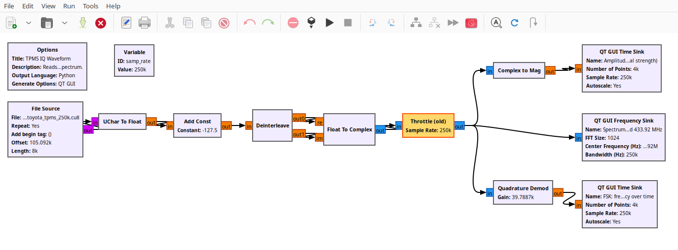The GNU Radio flowgraph I used to look at a TPMS recording.

Here’s what each part does:

• File Source reads the .cu8 recording, one byte at a time.
• UChar To Float and Add Const turn the bytes into numbers and centre them around zero. The RTL-SDR stores values from 0 to 255, so 127.5 is its zero.
• Deinterleave and Float To Complex split the stream back into I and Q and join them into one complex signal.
• Throttle plays the file back at the original speed, as if it were live.
• Then the signal goes three ways: Complex to Mag shows how strong the signal is, the frequency sink shows the spectrum, and Quadrature Demod shows how the frequency changes over time.

And this is what the Toyota sensor’s packet looks like:

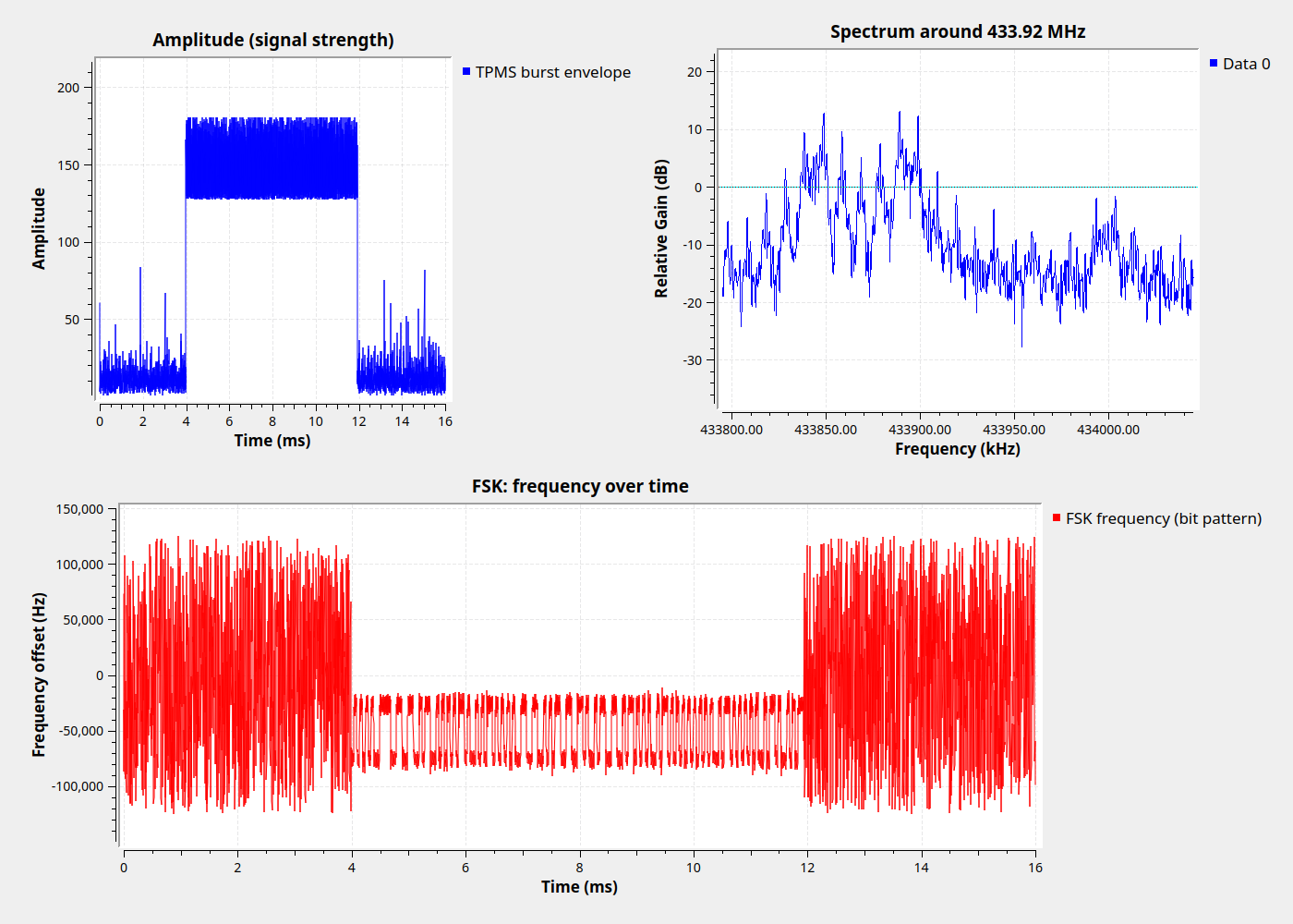One packet from a Toyota tyre sensor in GNU Radio. Signal: rtl_433 test collection.

The amplitude plot (top left) shows the packet. For about 8 milliseconds, the signal jumps up from the background noise, and that’s the whole packet.

The other two plots show that the sensor sends its data using something called FSK (Frequency Shift Keying). You can see two bumps in the spectrum (top right), and the frequency jumping between two levels during the packet (bottom). That pattern is the data: the sensor ID, the pressure and the temperature.

So this is what rtl_433 sees every time a car passes by. In the next post, we will look at what FSK and modulation actually mean, and turn this signal into bits and bytes.

Coming up in this series:

• What modulation and FSK are, and turning the raw signal into bits and bytes
• Building a surveillance lab in my glovebox to collect data on every drive
• Why the sensor measures temperature
• Doing all kinds of data analysis on the data collected

Stay tuned.